Welcome to econistics.com a website of Econistics Research and Consulting. This blog is designed to address the dilemma of interpreting different forms of controlling variables.
Here this illustration will cover the three types of control variables which can be placed in the functional form in 3 ways.
| Placement in Functional Form | |||
| Type of Control variable | Intercept Changing | Slope Changing | Both |
| Discrete Qualitative Control variable | Simple dummy | Interactive dummy | Interactive dummy |
| Continuous Qualitative control variable | Trend variable | Trend cross product | Trend and trend cross product |
| Quantitative Control Variable | Simple independent variable | Cross product | Moderator regression (both) |
| Quantitative Control Variable (Self) Special case | Square Form |
Before explaining this lets build one example as a base where there is one dependent variable and one independent variable. The example under discussion is the model of labor supply where the dependent variable is labor working hours and the independent variable is wage rate.

Qualitative Control Variable
Intercept changing case
Consider in a cross section model of labor supply you add a dummy variable of gender
Ls = a + b1 WH + b2 D + e
where D = 0 for Female & D = 1 for Male
For the case of b2 > 0 it is indicating that males are experiencing higher value of intercept i.e. a + b1
This is shown in the figure where when D = 1 the regression line shifts parallel upward. This means that for each value of wage rate there is a high supply of labor hours.

Slope changing case
consider a case of promotion of a fixed percentage for a worker it will increasingly increase the supply of working hours
Ls = a + b1 Wh + b2 D * Wh + e
where D = 1 for promoted worker & D = 0 for non-promoted worker
Here when D = 1 the slope gets increased to b1 + b2. This means that with the increase with the wage rate there is increasing number of working hours. The difference with previous case is that here the slope has increased and the gap between previous case (blue) and present case (red) is increasing with wage.

Intercept and Slope Changing case
Consider a case of a motivated worker who is supplying more hours but with increase in wages his propensity to provide more hours is also higher
Ls = a + b1 Wr + b2 D + b3 D * Wr + e
D = 1 for motivated worker & D = 0 for non-motivated worker
Here when D = 1 the intercept is increased to a + b2 and slope is increased to b1 + b3. This is because at start motivated worker is already providing more working hours but with the increase in the wage rate worker is willing to provide more hours.

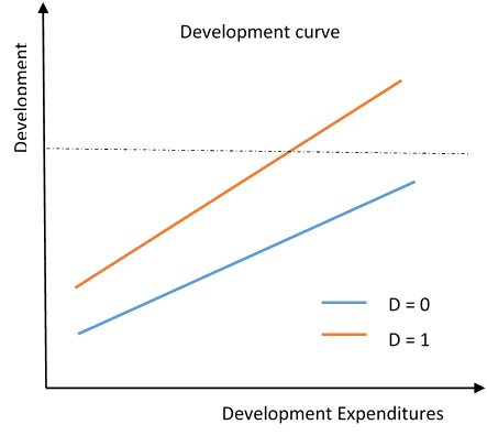
Application
The practical application of this illustration is the case where one want to explore the relationship between development and development expenditures but in a simple model the increase in the development expenditures are not creating enough development to achieve the SDG target. Here one can add a control variable of democracy v autocracy and see whether shifting from autocracy to democracy may shift the positively sloped graph upward lead it to achieve the SDG Target. The illustration is shown below.
Presentation in graphs
Now the challenge is while we have estimated the functional form. We need to draw the graphs as shown above. There is simple solution for this provided by Jeremy Dawson. In this link there is one excel file in which you have to provide the values of a, b1, b2 respectively, and it will draw the graph.
Keep following for more cases of specification of dummy variables. Like and participate at Econistics at facebook